Bringing Vector Search to the Lakehouse with Apache Hudi

TL;DR

AI applications increasingly need to search data by meaning, not just by exact fields or keywords. Product descriptions, support tickets, documents, images, and other unstructured data are becoming first-class inputs to analytics and application workflows. But adding semantic search to lakehouse data has usually meant introducing a separate vector database, copying embeddings into it, and maintaining a sync pipeline to keep records, metadata, deletes, and updates aligned.

Apache Hudi's native vector search brings that workflow closer to the table itself. Embeddings can live in the same Hudi table as the rest of the row, represented as a first-class VECTOR column and queried directly from SQL. This lets semantic search compose with structured filters, joins, updates, time travel, and incremental queries instead of requiring a separate sidecar system.

Hudi exposes vector search through two SQL functions: hudi_vector_search for a single query vector and hudi_vector_search_batch for running top-k search across a table of query vectors. Embeddings can be stored as FLOAT, DOUBLE, or INT8, and compared using cosine, L2, or dot product distance. The initial implementation uses distributed brute-force KNN, while an optimized ANN vector index is being developed behind the same SQL interface so applications can adopt the API today and benefit from faster algorithms as they land.

What is Semantic search?

Consider an example of a user interacting with an ecommerce site that has millions of product listings. Typically in most data analytics systems, a user would have to craft a query on exact fields, such as category, brand, price, size, or inventory_status in order to find a match.

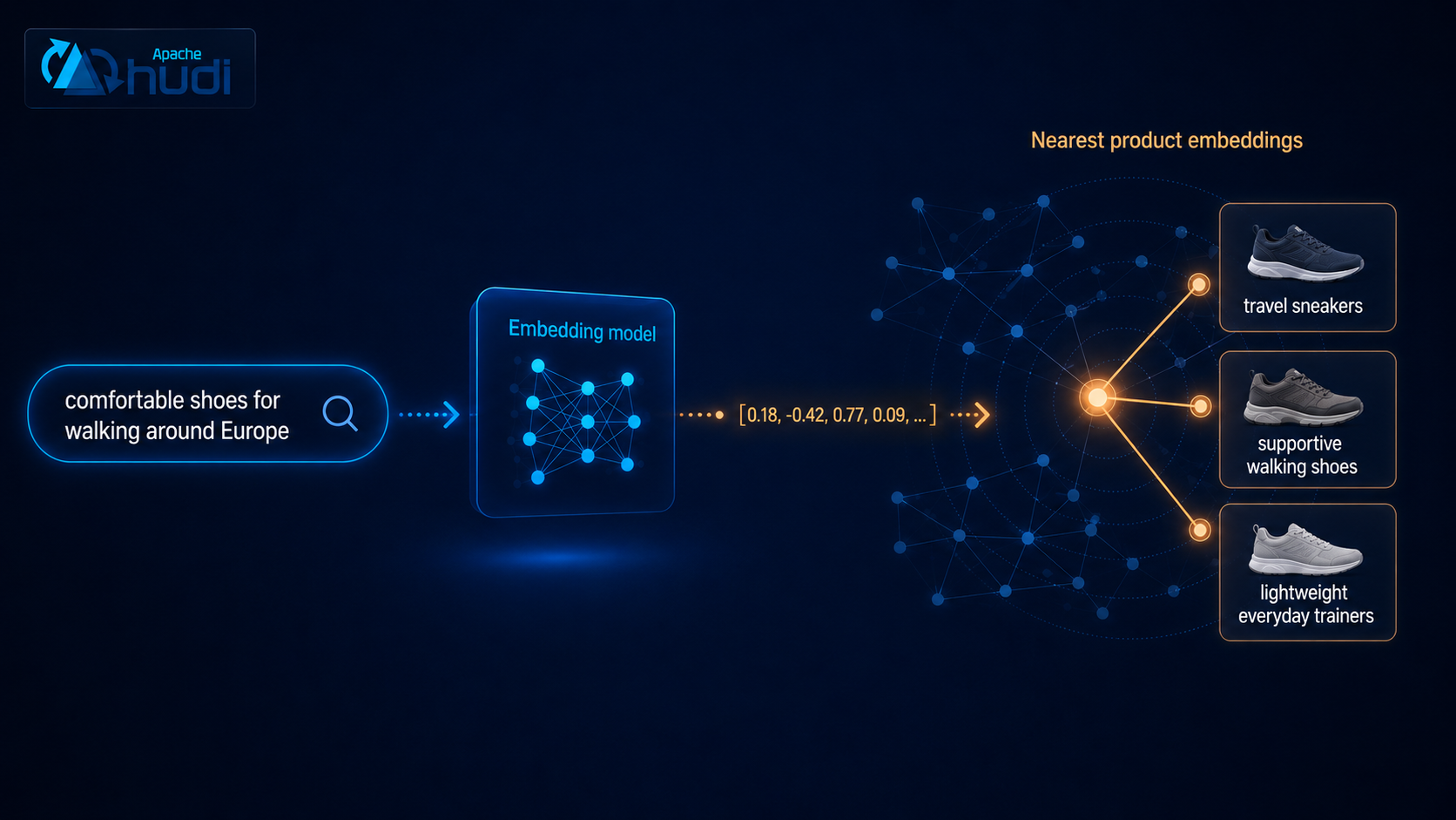
But many searches start with intent, and not direct fields. A user instead might search for "comfortable shoes for walking around Europe," even though there is no column called comfortable and no guarantee that the best listings use those exact words. Some products may say "travel sneakers," "all-day support," or "lightweight walking shoes" instead.

To handle this, semantic search is a way to search by meaning rather than by exact fields or keywords. It works by converting text, images, or other content into what are known as "vector embeddings".

A vector embedding is a fixed-size array of numbers that represents the meaning of some piece of data, such as a product description, customer review, image, support message, or document chunk.

Embeddings are typically produced by machine learning models. For text, this might be an embedding model or LLM-based encoder that converts a sentence, paragraph, or document chunk into a vector. For images, it might be a vision model that converts visual content into the same kind of numerical representation.

For example, a marketplace product description like:

Lightweight sneakers with cushioned soles for all-day walking

might be converted into a vector that looks conceptually like this:

[0.12, -0.03, 0.44, ..., 0.08]

The individual numbers in an embedding are often called features. Each one helps place the original item somewhere in a high-dimensional space. For a product description, the model may learn features related to things like product type, use case, style, material, comfort, or activity. For an image, the features may capture patterns related to shape, color, texture, or visual similarity.

These features are usually not directly interpretable on their own. One number does not simply mean "comfort" or "travel." Instead, the full vector captures many learned signals together. What matters is how one vector relates to another. Products with similar meaning should produce vectors that are close together, even if the words are different.

That is what allows a search like "comfortable shoes for walking around Europe" to match products described as "travel sneakers," "supportive walking shoes," or "lightweight everyday trainers," even when those listings do not use the exact same words as the query.

The need for both structured and unstructured data

The marketplace example shows why modern AI applications need both unstructured and structured data. The meaning of a product may live in descriptions, reviews, images, or support conversations, which can be converted into embeddings and searched semantically. But deciding whether a result is useful still depends on structured fields such as price, size, inventory_status, shipping_region, and seller_rating.

This pattern has become more important with the rise of LLM-powered applications. Search, recommendations, RAG, document intelligence, and agent workflows increasingly operate over text, images, and other unstructured data. But these applications still need the guarantees of structured data systems: filters, joins, updates, deletes, freshness, and governance.

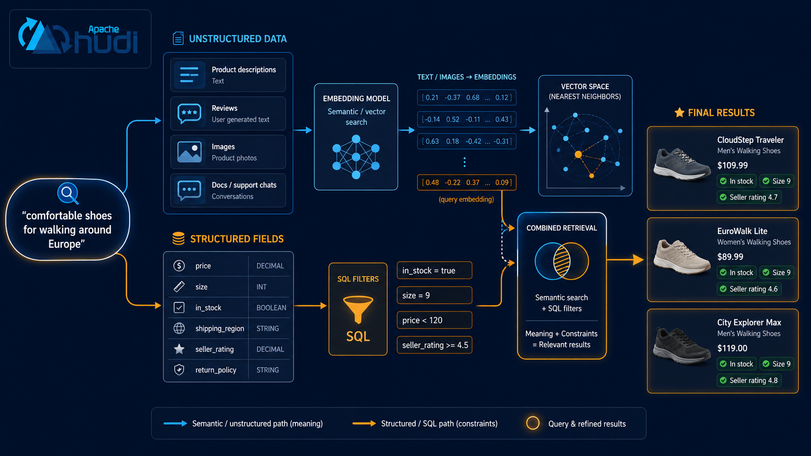
This is where the lakehouse becomes a natural fit. In many AI applications, the embedding is not an independent object. It is derived from the row itself: a product description, review, image, support conversation, document chunk, or some combination of fields. When that source data changes, the embedding needs to change with it. When a row is deleted, expired, corrected, or reprocessed, the corresponding embedding needs to follow the same lifecycle.

A standalone vector database can be a good serving layer, especially for ultra-low-latency retrieval at very large scale. But if the source records live in the lakehouse, a separate vector database introduces another copy of the data. That copy has to be kept in sync with the table, including inserts, updates, deletes, schema changes, metadata filters, and backfills. Over time, the hard problem becomes less about computing nearest neighbors and more about maintaining consistency between the source data and the vector index.

Hudi vector search is built around a simpler model: keep the original records, structured metadata, and embeddings together in the same table. In an ingestion pipeline, new and changed records can be processed incrementally, embeddings can be generated or refreshed from the latest source fields, and both the source data and vector columns can be committed together into Hudi. That makes the Hudi table the single source of truth for both analytics and semantic search.

For example, Hudi Streamer can ingest changes from sources such as Kafka or cloud storage into a Hudi table. An embedding step can be added to the pipeline so that when product descriptions, reviews, images, or metadata change, the corresponding embeddings are updated as part of the same table workflow.

How does Hudi represent VECTOR?

Once embeddings are produced, they need to be stored in a table in a way that preserves their meaning. A plain array of numbers can store the values, but it does not tell the table system that the column is a fixed-dimensional vector intended for similarity search.

Hudi represents embeddings using a first-class logical type: VECTOR(dimension) or VECTOR(dimension, element_type). The dimension value defines the fixed length of the vector. For example, VECTOR(768) represents an embedding with 768 values.

A product catalog table can declare a vector column directly in SQL DDL:

CREATE TABLE products (
  product_id string,
  title string,
  category string,
  brand string,
  price double,
  inventory_status string,
  description string,
  description_embedding VECTOR(768)
) USING hudi;

When the element type is omitted, Hudi uses FLOAT by default. This is the most common representation for embeddings produced by text and image models. Hudi also supports DOUBLE and INT8 for workloads that need higher precision or more compact storage.

The storage difference becomes meaningful at scale. A VECTOR(768, FLOAT) stores 3,072 bytes of raw vector values per row. The same vector represented as INT8 stores 768 bytes per row. Across millions or billions of rows, that difference affects table size, index size, and query cost.

At the Hudi table level, both the SQL DDL form and the DataFrame API form describe the same logical column: a fixed-dimensional vector that can be validated, indexed, and used for vector search. At the physical storage layer, Hudi maps the logical vector type onto storage formats in a way that balances efficiency and interoperability. Readers that do not understand the Hudi vector logical type can still access the underlying data, while Hudi-aware readers can validate dimensions and treat the column as a single vector value. The DataFrame API equivalent and on-disk encoding are covered in the docs.

Today, vector columns are supported as top-level columns. They cannot yet be nested inside structs, arrays, or maps. For data models that naturally contain multiple embeddings per entity, such as a product with many variants, the current pattern is to model each embedded item as its own row. Nested vector support can be added in the future as the type system and query semantics evolve.

Querying with Hudi Vector Search

Once embeddings are stored in a Hudi table, they can be searched directly from SQL. Hudi provides two table-valued functions:

• hudi_vector_search for one query vector
• hudi_vector_search_batch for many query vectors

The difference is easiest to understand through the marketplace example.

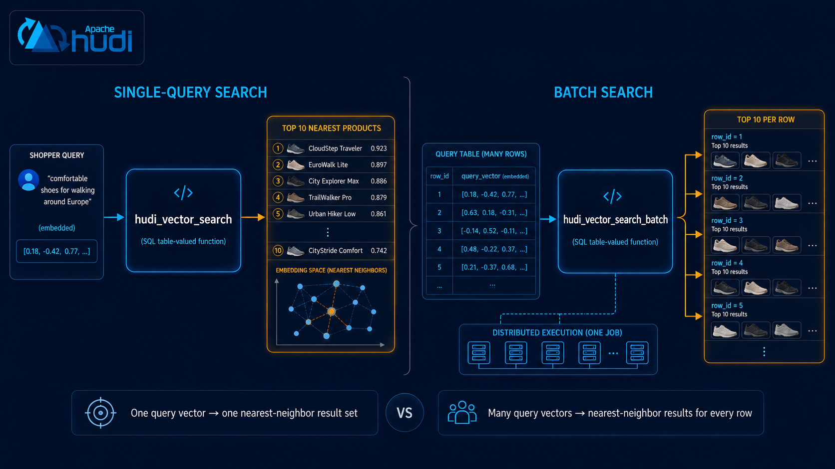
A single-query search answers a question like: Given this shopper query, find the 10 most similar products.

A batch search answers a larger version of the same question: Given this table of many shopper queries, products, or documents, find the 10 most similar products for each row.

So single-query search is one nearest-neighbor lookup. Batch search is the same lookup repeated for every row in another table, executed as one distributed job.

Single-query vector search

hudi_vector_search takes the table to search, the embedding column, a query vector, and k, plus a few optional arguments: the distance metric (cosine, l2, or dot_product), a filter predicate applied before distance computation, and a max_distance cutoff to drop weak matches. For a full list of parameters refer to the following docs.

For example, a shopper might search for "wireless headphones for travel." The application converts that text into an embedding and searches the product catalog:

SELECT product_id, title, brand, price, _hudi_distance
FROM hudi_vector_search(
  'product_embeddings',
  'embedding',
  ARRAY(/* embedding of the shopper query */),
  10,
  'cosine',
  'brute_force',
  'category = ''electronics'' AND in_stock = true',
  0.4
);

The filter is important. Since the first implementation uses brute-force search, reducing the candidate set before distance computation is one of the most effective ways to control latency. Searching 50 million product embeddings is expensive. Searching only the in-stock electronics products may reduce the search space to a much smaller subset.

The max_distance argument is another practical control. It removes results whose distance is above the threshold, so the query does not return weak or irrelevant matches simply to fill the requested k.

The output includes all corpus columns except the embedding column, plus _hudi_distance. Results are ordered by distance ascending, so smaller values are more similar.

Batch Vector Search

Batch search is useful when you do not have just one query. Instead, you have a whole table of things that each need their own nearest-neighbor results.

That is what hudi_vector_search_batch does: it runs top-k vector search for every row in a query table. It takes the same arguments as the single-query form, but searches with a whole query_table (and its query_col) instead of a single vector, returning the top k corpus rows for each query row. See the docs for the full signature.

For example, suppose a marketplace wants to precompute related products every night. The input is not one shopper query. The input is a table of products:

SELECT
  query_product_id,
  product_id AS related_product_id,
  title,
  _hudi_distance,
  _hudi_query_index
FROM hudi_vector_search_batch(
  'product_embeddings',
  'embedding',
  'query_products',
  'query_embedding',
  20,
  'cosine',
  'brute_force',
  'in_stock = true',
  0.4
);

The result contains the matching corpus rows, the query row metadata, and the computed distance. Hudi omits the embedding columns from the output because applications usually need the matching records and scores, not the raw vectors.

Batch search also adds _hudi_query_index, which identifies which query row produced each result. This is useful because the output contains many groups of top-k results: one group per query row.

Put simply:

• hudi_vector_search returns the nearest rows for one query.
• hudi_vector_search_batch returns the nearest rows for each query in a query table.

Batch search is especially useful for offline or scheduled workloads: related-product generation, duplicate detection, content matching, recommendation refreshes, and document similarity jobs.

How the brute-force implementation works

The previous section introduced the SQL interface for single-query and batch vector search. The next natural question is: what happens when those queries run?

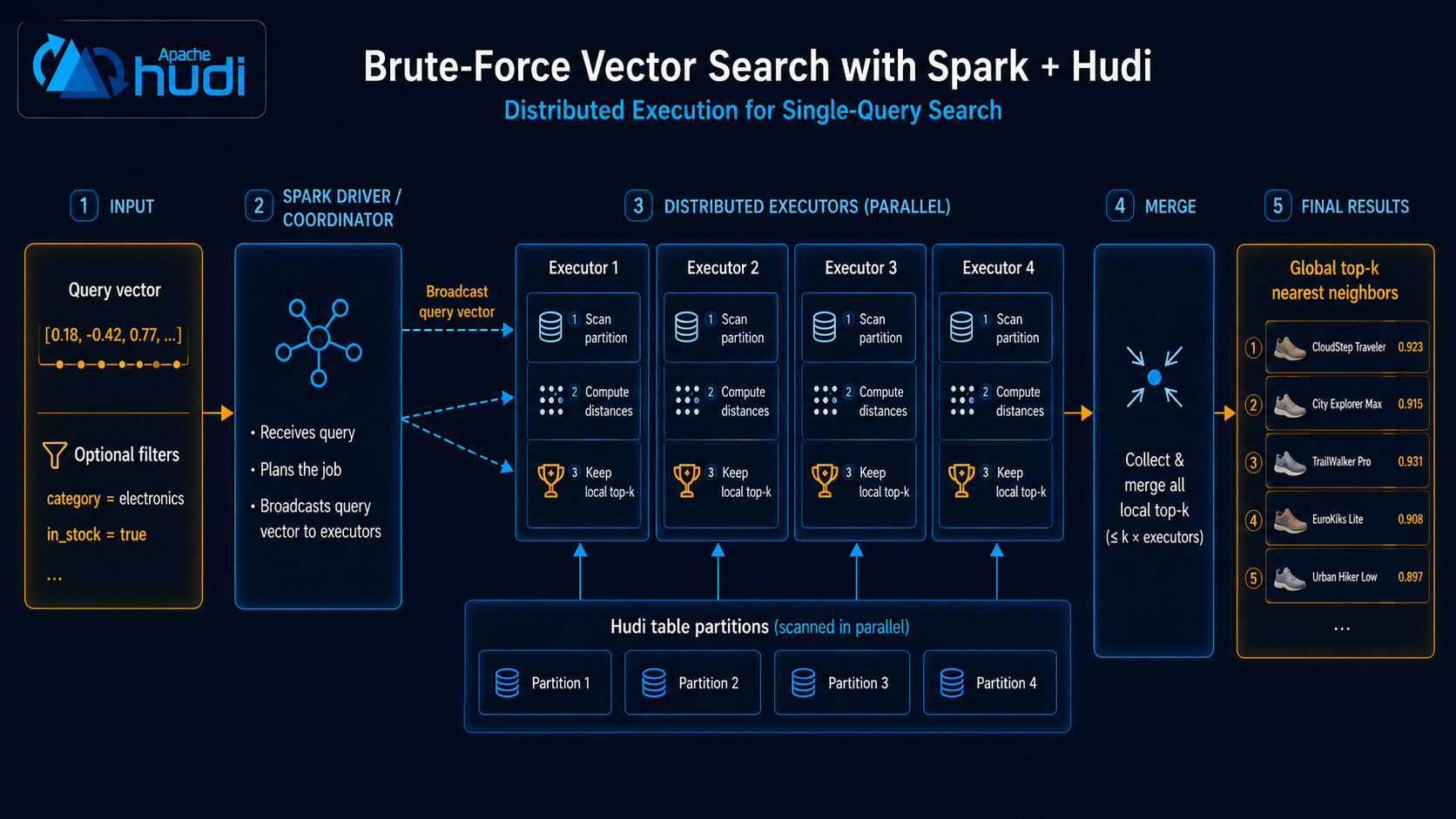
For a single-query search, the execution flow is:

1. Spark receives the query vector and broadcasts it to executors.
2. Each executor scans its portion of the corpus.
3. For each row, the executor computes the distance between the query vector and the row's embedding.
4. Each executor keeps only its local top k matches.
5. The driver merges those local top-k results into the final global top-k result.

This keeps executor memory bounded by k, rather than by the total size of the corpus. Even if an executor scans millions of rows, it only needs to keep the best candidates it has seen so far.

The main cost is distance computation. If the query searches 50 million embeddings, Hudi has to compare the query vector against 50 million candidate vectors. If the query first filters the corpus down to 200,000 relevant rows, the amount of distance computation drops dramatically.

That is why the filter argument in hudi_vector_search matters. It lets applications apply structured predicates before vector distance computation runs. For example, an ecommerce query may search only products where category = 'electronics' and in_stock = true, rather than searching the entire product catalog.

Batch search follows the same idea, but repeats it for many query vectors in one distributed job. Instead of asking, "what are the nearest products for this one shopper query?", batch search asks, "what are the nearest products for every row in this query table?"

For example, a nightly recommendation job might take every active product as a query row and find the top 20 related products for each one. Hudi compares each query embedding against the filtered corpus, ranks matches per query, and returns one group of top-k results for each query row.

Because batch search multiplies the amount of work by the number of query rows, the candidate set matters even more. A small query table searched against a well-filtered corpus can be practical. A large query table searched against an unfiltered corpus can become expensive quickly. This is why batch search is best suited for offline or scheduled workloads such as related-product generation, duplicate detection, content matching, and recommendation refreshes.

The max_distance argument is useful in both single-query and batch search. It removes weak matches above a distance threshold before returning results. In batch jobs, this can reduce output size significantly because each query row may otherwise produce up to k results, even when some matches are not useful.

This is why vector search becomes more powerful when it is integrated with table semantics. Many applications do not want nearest neighbors across all data. They want nearest neighbors within a meaningful slice of the table: active products, recent documents, records for a specific customer, listings in a region, or items that pass business rules. It is most useful when combined with the same filtering, pruning, and table layout techniques that data systems already use to reduce the amount of data read.

Future Vector index

The SQL interface is designed to stay stable as new algorithms are added. Today, algorithm => 'brute_force' uses a distributed linear scan. In the future, indexed implementations such as IVF-PQ can replace the scan with an index lookup plan.

In that model, Hudi would use a vector index to produce candidate record IDs and distances, then join those candidates back to the table to return the same output shape. Applications written against the current table-valued function interface should not need to change when switching from brute-force search to indexed search.

Conclusion

For the past few years, adding semantic search to a lakehouse application usually meant adding a separate vector database, copying embeddings into it, and maintaining a sync pipeline between the two systems. That architecture works, but it adds operational complexity at exactly the point where correctness matters: keeping records, embeddings, metadata, deletes, and updates aligned.

Hudi vector search takes a different approach. Embeddings are stored in the same table as the rest of the row, with the same schema, snapshots, updates, and table services. Vector search becomes part of the query layer instead of a separate sidecar system that has to be synchronized with the lakehouse.

The first implementation focuses on making this model simple and usable: a VECTOR type for embeddings, SQL functions for single-query and batch vector search, and integration with Hudi's existing table semantics. This is especially useful for RAG, document intelligence, recommendation refreshes, deduplication, clustering, and similarity search jobs where correctness, freshness, and SQL composability matter as much as raw serving latency.

The best way to understand the model is to try it directly. Start with Hudi 1.2, create a table with a VECTOR column, load a small set of embeddings, and run your first hudi_vector_search query. From there, try adding structured filters, experimenting with hudi_vector_search_batch, or materializing similarity results back into a Hudi table.

If you are building AI applications on lakehouse data, this is the core idea to test: semantic search does not have to live outside the table. With Hudi, embeddings, metadata, updates, and search can move through the same data system.